38 edit labels in excel chart

Excel tutorial: How to customize axis labels Instead you'll need to open up the Select Data window. Here you'll see the horizontal axis labels listed on the right. Click the edit button to access the label range. It's not obvious, but you can type arbitrary labels separated with commas in this field. So I can just enter A through F. When I click OK, the chart is updated. How to Change the Y Axis in Excel - Alphr Click the dropdown next to "Display Units," then make your selection such as "millions" or "hundreds." To label the displayed units, go to the "Axis Options -> Display units" section. Add a...

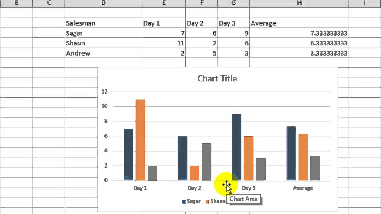
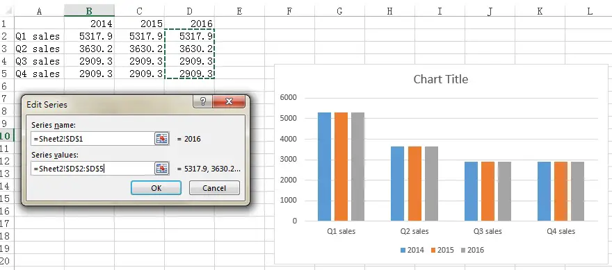
How to rename a data series in an Excel chart? To rename a data series in an Excel chart, please do as follows: 1. Right click the chart whose data series you will rename, and click Select Data from the right-clicking menu. See screenshot: 2. Now the Select Data Source dialog box comes out. Please click to highlight the specified data series you will rename, and then click the Edit button. See screenshot:

Edit labels in excel chart

Custom Excel Chart Label Positions • My Online Training Hub The alternate method is to add the labels to the ghost series, and then manually assign the actual value cells, one by one, to the labels by clicking each one twice (slowly, not a double click) to select the individual label > click in the formula bar and type = then click on the cell that contains the actual value for that label. How to Change Excel Chart Data Labels to Custom Values? You can change data labels and point them to different cells using this little trick. First add data labels to the chart (Layout Ribbon > Data Labels) Define the new data label values in a bunch of cells, like this: Now, click on any data label. This will select "all" data labels. Now click once again. Edit titles or data labels in a chart - support.microsoft.com To edit the contents of a title, click the chart or axis title that you want to change. To edit the contents of a data label, click two times on the data label that you want to change. The first click selects the data labels for the whole data series, and the second click selects the individual data label.

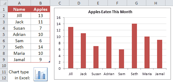
Edit labels in excel chart. Change axis labels in a chart - support.microsoft.com Right-click the category labels you want to change, and click Select Data. In the Horizontal (Category) Axis Labels box, click Edit. In the Axis label range box, enter the labels you want to use, separated by commas. For example, type Quarter 1,Quarter 2,Quarter 3,Quarter 4. Change the format of text and numbers in labels Excel charts: add title, customize chart axis, legend and ... To change what is displayed on the data labels in your chart, click the Chart Elements button > Data Labels > More options… This will bring up the Format Data Labels pane on the right of your worksheet. Switch to the Label Options tab, and select the option (s) you want under Label Contains: How do I modify Excel Chart data point PopUp's? Hi, Based on my understanding, I think you want to modify/add the tooltip text of the point in your XY scatter charts without the data labels. As for as I know, there is no property and method of Chart object to edit the tooltip of the Chart point in Excel Object Model. However, you could use VBA programming to simulate the feature, although it is by no means a simple task. How to edit the label of a chart in Excel? - Stack Overflow The latter box will list the "1", "2", etc. numbers that you want to change. Hit the edit button for the right-hand box (Horizontal Category (Axis) Labels), and you will be prompted to enter an axis label range. Instead of selecting a range, though, just enter the labels that you want to see on the x-axis, separated by commas, like so: Press OK, and then again when the Select Data Source dialogue reappears, and it's done.

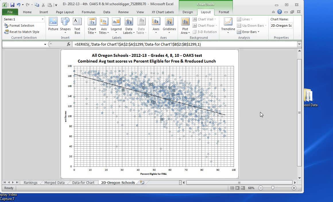
How to Create and Customize a Waterfall Chart in Microsoft ... Select the chart and use the buttons on the right (Excel on Windows) to adjust Chart Elements like labels and the legend, or Chart Styles to pick a theme or color scheme. Select the chart and go to the Chart Design tab. How to Insert Axis Labels In An Excel Chart | Excelchat We will go to Chart Design and select Add Chart Element Figure 6 - Insert axis labels in Excel In the drop-down menu, we will click on Axis Titles, and subsequently, select Primary vertical Figure 7 - Edit vertical axis labels in Excel Now, we can enter the name we want for the primary vertical axis label. Change Chart Axis Labels to 1st of Each Month [SOLVED] Re: Change Chart Axis Labels to 1st of Each Month. Based on those pictures it looks like you are using an XY scatter chart, which does not have the same "category/date axis" options like you saw described in the help file. In order to get those options, you need to change your chart type to line and make sure that Excel designates the ... How to Edit Legend in Excel - Excelchat Change Series Name in Select Data Step 1. Right-click anywhere on the chart and click Select Data Figure 4. Change legend text through Select Data Step 2. Select the series Brand A and click Edit Figure 5. Edit Series in Excel The Edit Series dialog box will pop-up. Figure 6. Edit Series preview pane Step 3.

How do I resize data labels in Excel 2010 ... How do I change data labels to percentages in Excel pie chart? Right click the pie chart again and select Format Data Labels from the right-clicking menu. 4. In the opening Format Data Labels pane, check the Percentage box and uncheck the Value box in the Label Options section. Then the percentages are shown in the pie chart as below screenshot ... Excel 2010: How to format ALL data point labels ... I want to change the format (I.E. enlarge, etc.) my data point labels all at the same time. But when I select "More Data Label Options" under the layout ribbon's Data Label menu, Excel automatically selects my first data point label (even if I have the whole graph selected). Is there any way to format all data labels simultaneously in Excel 2010? How to Use Cell Values for Excel Chart Labels Select the chart, choose the "Chart Elements" option, click the "Data Labels" arrow, and then "More Options." Uncheck the "Value" box and check the "Value From Cells" box. Select cells C2:C6 to use for the data label range and then click the "OK" button. The values from these cells are now used for the chart data labels. How to Customize Your Excel Pivot Chart Data Labels - dummies The Data Labels command on the Design tab's Add Chart Element menu in Excel allows you to label data markers with values from your pivot table. When you click the command button, Excel displays a menu with commands corresponding to locations for the data labels: None, Center, Left, Right, Above, and Below. None signifies that no data labels should be added to the chart and Show signifies ...

Excel Course: Inserting Graphs

How to Change Horizontal Axis Labels in Excel 2010 - Solve ... How to Edit Horizontal Axis Labels in Microsoft Excel 2010 Most of the benefit that comes from using the chart creation tool in Microsoft Excel lies with the one click process of creating the chart, but it is actually a fully-featured utility that you can use to customize the generated chart in a number of different ways.

Charts and Graphs in Excel

How To Modify A Chart in Microsoft Excel? | Smart Office Once selected, the Change Chart Type dialog box appears as shown, with all the Charts available to use. Once we have decided which Chart to use, we press the Ok button, and the Chart has changed and updated. The final command that is available on the Chart Design Tab and that is located at the far-right area of the ribbon named Location and is Move Chart will be described later. As mentioned, everything depends on the Data. What we want to visualize and how we want to visualize it, does not ...

How to change x axis values in Microsoft excel - YouTube

Creating and Modifying Charts - Using Microsoft Excel ... In all cases, you have to select the chart first to access Chart Tools. To add any labels (for example, the title or axes), under the Design ribbon, click Add Chart Element in the Chart Layouts group and select the desired label. To change the chart type, data, or location, use the Chart Tools Design ribbon.

X-Y Chart (Excel 2010) - Step 2 Construct a Scatter Chart with Labels - YouTube

How to Rename a Legend in an Excel Chart To do this, click on the chart, then find the tab ' Chart Design ' and go for the option ' Select Data '. You'll see a pop-up window where you can easily edit the information from the legend. Here we'll focus on the left-hand side of the window and click on ' Sales ', then on ' Edit '.

Making interactive charts in Excel - A case study with gender equality gap data - Advanced ...

Excel VBA Chart Data Label Font Color in 4 Easy Steps ... In this Excel VBA Chart Data Label Font Color Tutorial, you learn how to change a Chart's Data Label(s) font color with Excel macros.. This Excel VBA Chart Data Label Font Color Tutorial: Applies to Data Labels in a Chart. Doesn't apply to the following: ActiveX Labels in a worksheet.

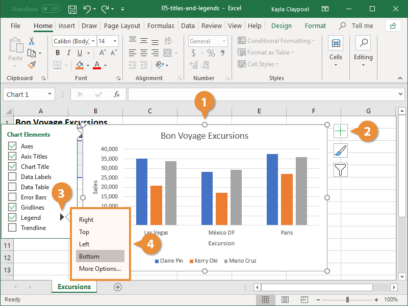
How to Edit a Legend in Excel | CustomGuide

editing Excel histogram chart horizontal labels ... On the one hand, since you have found the workaround, we'd suggest you use the workaround. On the other hand, if you want to use such chart, you can also create bar chart. However, you may need to calculate the number of those data, then you can insert bar chat. And it will show the effect you want.

Multiple Series in One Excel Chart - Peltier Tech Blog

Εισαγωγή στο SPSS, Ενότητα 1 - Πανεπιστήμιο Πειραιώς το «female» (μέχρι 60 χαρακτήρες) (για να εμφανίζονται στον Data editor τα value labels αντί των πραγ- ματικών τιμών των μεταβλητών επιλέγουμε από το menu: ...13 σελίδες

Excel clustered column chart - Access-Excel.Tips

How to change chart axis labels' font color and size in Excel? Just click to select the axis you will change all labels' font color and size in the chart, and then type a font size into the Font Size box, click the Font color button and specify a font color from the drop down list in the Font group on the Home tab. See below screen shot:

Share :