45 how to add data labels to a 3d pie chart in excel

How to Show Percentage in Pie Chart in Excel? - GeeksforGeeks Jun 29, 2021 · Select a 2-D pie chart from the drop-down. A pie chart will be built. Select -> Insert -> Doughnut or Pie Chart -> 2-D Pie. Initially, the pie chart will not have any data labels in it. To add data labels, select the chart and then click on the “+” button in the top right corner of the pie chart and check the Data Labels button. How to Create a Pie Chart in Excel in 60 Seconds or Less - HubSpot Create your columns and/or rows of data. Feel free to label each column of data — excel will use those labels as titles for your pie chart. Then, highlight the data you want to display in pie chart form. 2. Now, click "Insert" and then click on the "Pie" logo at the top of excel. 3.

Excel 3-D Pie charts - Microsoft Excel 2016 - OfficeToolTips 2. On the Insert tab, in the Charts group, choose the Pie button: Choose 3-D Pie. 3. Right-click in the chart area, then select Add Data Labels and click Add Data Labels in the popup menu: 4. Click in one of the labels to select all of them, then right-click and select Format Data Labels... in the popup menu: 5.

How to add data labels to a 3d pie chart in excel

Excel charts: add title, customize chart axis, legend and data labels Select the chart and go to the Chart Tools tabs ( Design and Format) on the Excel ribbon. Right-click the chart element you would like to customize, and choose the corresponding item from the context menu. Use the chart customization buttons that appear in the top right corner of your Excel graph when you click on it. How to Make a Pie Chart in Excel (Only Guide You Need) 13.07.2022 · Read More: How to Make a Pie Chart in Excel with One Column of Data. How to Modify/Edit the Pie Chart. To modify or edit an Excel pie chart you need to select the pie chart 1 st. After selecting the chart, you will find 3 options just beside it. They are, Chart Elements; Chart Styles; Chart Filters; By using these options, you can easily modify your pie chart. # Adding … Edit titles or data labels in a chart - support.microsoft.com The first click selects the data labels for the whole data series, and the second click selects the individual data label. Click again to place the title or data label in editing mode, drag to select the text that you want to change, type the new text or value.

How to add data labels to a 3d pie chart in excel. Display data point labels outside a pie chart in a paginated report ... Create a pie chart and display the data labels. Open the Properties pane. On the design surface, click on the pie itself to display the Category properties in the Properties pane. Expand the CustomAttributes node. A list of attributes for the pie chart is displayed. Set the PieLabelStyle property to Outside. Set the PieLineColor property to Black. How to Create a Pie Chart in Excel | Smartsheet Enter data into Excel with the desired numerical values at the end of the list. Create a Pie of Pie chart. Double-click the primary chart to open the Format Data Series window. Click Options and adjust the value for Second plot contains the last to match the number of categories you want in the "other" category. How to Show Percentage in Excel Pie Chart (3 Ways) Sep 08, 2022 · Display Percentage in Pie Chart by Using Format Data Labels. Another way of showing percentages in a pie chart is to use the Format Data Labels option. We can open the Format Data Labels window in the following two ways. 2.1 Using Chart Elements. To active the Format Data Labels window, follow the simple steps below. Steps: How to Rotate Pie Chart in Excel? - WallStreetMojo Move the cursor to the chart area to select the pie chart. Step 5: Click on the Pie chart and select the 3D chart, as shown in the figure, and develop a 3D pie chart. Step 6: In the next step, change the title of the chart and add data labels to it. Step 7: To rotate the pie chart, click on the chart area.

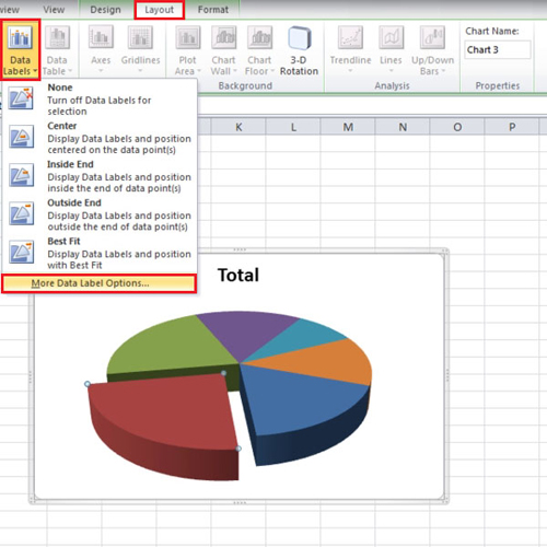
3D Plot in Excel | How to Plot 3D Graphs in Excel? - EDUCBA For that, select the data and go to the Insert menu; under the Charts section, select Line or Area Chart as shown below. After that, we will get the drop-down list of Line graphs as shown below. From there, select the 3D Line chart. After clicking on it, we will get the 3D Line graph plot as shown below. How to Make a Pie Chart in Excel & Add Rich Data Labels to The Chart! 7) With the data point still selected, go to Chart Tools>Format>Shape Styles and click on the drop-down arrow next to Shape Effects and select Shadow and choose Inner Shadow>Inside Diagonal Top Left. 8) With the one data point still selected, right-click this data point, and select Add Data Label>Add Data Callout as shown below. Create a Pie Chart in Excel (In Easy Steps) - Excel Easy Create the pie chart (repeat steps 2-3). 7. Click the legend at the bottom and press Delete. 8. Select the pie chart. 9. Click the + button on the right side of the chart and click the check box next to Data Labels. 10. Click the paintbrush icon on the right side of the chart and change the color scheme of the pie chart. How to Add Data Labels to an Excel 2010 Chart - dummies On the Chart Tools Layout tab, click Data Labels→More Data Label Options. The Format Data Labels dialog box appears. You can use the options on the Label Options, Number, Fill, Border Color, Border Styles, Shadow, Glow and Soft Edges, 3-D Format, and Alignment tabs to customize the appearance and position of the data labels.

PIE CHART in R with pie() function [WITH SEVERAL EXAMPLES] An alternative to display percentages on the pie chart is to use the PieChart function of the lessR package, that shows the percentages in the middle of the slices.However, the input of this function has to be a categorical variable (or numeric, if each different value represents a category, as in the example) of a data frame, instead of a numeric vector. Excel 3-D Pie charts - Microsoft Excel 365 - OfficeToolTips 2. On the Insert tab, in the Charts group, choose the Pie button: Choose the 3-D Pie chart. 3. Right-click in the chart area, then select Add Data Labels and click Add Data Labels in the popup menu: 4. Click in one of the labels to select all of them, then right-click and select Format Data Labels... in the popup menu. 5. How to add data labels from different column in an Excel chart? Click any data label to select all data labels, and then click the specified data label to select it only in the chart. 3. Go to the formula bar, type =, select the corresponding cell in the different column, and press the Enter key. See screenshot: 4. Repeat the above 2 - 3 steps to add data labels from the different column for other data points. Pie Chart Examples | Types of Pie Charts in Excel with Examples It is similar to Pie of the pie chart, but the only difference is that instead of a sub pie chart, a sub bar chart will be created. With this, we have completed all the 2D charts, and now we will create a 3D Pie chart. 4. 3D PIE Chart. A 3D pie chart is similar to PIE, but it has depth in addition to length and breadth.

How to Create and modify a pie chart in Excel | HowTech

how to create a shaded range in excel — storytelling with data 08.10.2019 · Add a new data series for the Minimum by right-clicking the chart and choosing “Select Data”: In the Select Data Source dialog box, click the + button to add a new data series for the Minimum (my Min series is in cells O6:O17 with Name in O5).

How to Create and Format a Pie Chart in Excel

Add or remove data labels in a chart - support.microsoft.com Add data labels to a chart, Click the data series or chart. To label one data point, after clicking the series, click that data point. In the upper right corner, next to the chart, click Add Chart Element > Data Labels. To change the location, click the arrow, and choose an option.

Math Arguments: 83: Pie Chart

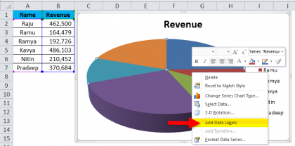
How To Make a Pie Chart in Excel (With Tips) | Indeed.com First, right-click on the pie chart and select "Add data labels" to insert the numerical value of each piece onto the pie chart. If you want your pieces to show category names, you can edit them by right-clicking any label and selecting "Format data labels," followed by "Label options."

3D Disk Pie Chart in Excel - PK: An Excel Expert

2D & 3D Pie Chart in Excel - Tech Funda To add filters to the Pie chart, click on the chart and select 'Chart Filters' command button at the top-right of the chart as dislayed in the picture below. To plot the Target data on the chart, select 'Target' series radio button and click 'Apply' button.

How to Create a Pie Chart in Microsoft Excel

How to make a 3D pie chart in Excel - Quora Answer (1 of 4): I have never been a fan of pie charts. Pie charts are intended to show the user group category percentages. Here is an example using Minitab and the tires.mtw data set. This is a pie chart of tire failures by category. In general, users have difficulty comparing percentages due ...

How to Make Pie Charts and Graphs in Excel - BSUPERIOR

How to insert data labels to a Pie chart in Excel 2013 - YouTube This video will show you the simple steps to insert Data Labels in a pie chart in Microsoft® Excel 2013. Content in this video is provided on an "as is" basi...

Pie Chart in Excel | How to Create Pie Chart | Step-by-Step Guide Chart

Solved Add Data Callouts as data labels to the 3-D pie - Chegg See the answer. Add Data Callouts as data labels to the 3-D pie chart. Include the category name and percentage in the data labels. Slightly explode the segment of the chart that was allocated the smallest amount of advertising funds. Adjust the rotation of the 3-D Pie chart with a X rotation of 20, a Y rotation of 40, and a Perspective of 10 .

Pie Chart in Excel | How to Create Pie Chart | Step-by-Step Guide Chart

How to ☝️Create A 3-D Pie Chart in Excel - SpreadsheetDaddy Right-click on your 3-D pie graph and click " Add Data Labels. ", Go to the Label Options tab. Check the " Category Name " box to display the names of the categories along with the actual market share data. Recolor the Slices, Next stop: changing the color of the slices.Double-click on the slice you want to recolor and select " Format Data Point.

Creating an Excel Pie Chart | 500 Rockets Marketing

Tips for turning your Excel data into PowerPoint charts 21.08.2012 · Limit the Data. Instead of creating a chart from data in an entire Excel spreadsheet, first edit your spreadsheet. One way to do this is to copy and paste data onto a separate Excel workbook tab. Then look at what you can eliminate. When you have only the data you need, you’re ready to create the chart in PowerPoint.

How to insert data labels in a Pie chart in Excel 2013 - YouTube

How to Make a Pie Chart with Multiple Data in Excel (2 Ways) - ExcelDemy First, to add Data Labels, click on the Plus sign as marked in the following picture. After that, check the box of Data Labels. At this stage, you will be able to see that all of your data has labels now. Next, right-click on any of the labels and select Format Data Labels. After that, a new dialogue box named Format Data Labels will pop up.

Vector Tutorial: Creating A Killer 3D Pie Chart in Illustrator | Designfreebies

Microsoft Excel Tutorials: Add Data Labels to a Pie Chart - Home and Learn To add the numbers from our E column (the viewing figures), left click on the pie chart itself to select it: The chart is selected when you can see all those blue circles surrounding it. Now right click the chart. You should get the following menu: From the menu, select Add Data Labels. New data labels will then appear on your chart:

How to Make a Pie Chart in Excel & Add Rich Data Labels to The Chart!

ggplot2 pie chart : Quick start guide - R software and data Customized pie charts. Create a blank theme : blank_theme . - theme_minimal()+ theme( axis.title.x = element_blank(), axis.title.y = element_blank(), panel.border = element_blank(), panel.grid=element_blank(), axis.ticks = element_blank(), plot.title=element_text(size=14, face="bold") ). Apply the blank theme; Remove axis tick mark labels; Add text annotations : The …

How to Make a Pie Chart in Excel & Add Rich Data Labels to The Chart!

Creating Pie Chart and Adding/Formatting Data Labels (Excel) Creating Pie Chart and Adding/Formatting Data Labels (Excel) Creating Pie Chart and Adding/Formatting Data Labels (Excel)

What do you mean I'm not supposed to use Pie Charts?! | Geckoboard blog

How to show data labels in charts created via Openpyxl 2 Answers. This works for me on a line chart (As a combination chart): openpyxls version: 2.3.2: from openpyxl.chart.label import DataLabelList chart2 = LineChart () .... code to build chart like add_data () and: # Style the lines s1 = chart2.series [0] s1.marker.symbol = "diamond" ... your data labels added here: chart2.dataLabels ...

Pie Chart in Excel | How to Create Pie Chart? (Types, Examples)

how to add data labels into Excel graphs — storytelling with data You can download the corresponding Excel file to follow along with these steps: Right-click on a point and choose Add Data Label. You can choose any point to add a label—I'm strategically choosing the endpoint because that's where a label would best align with my design. Excel defaults to labeling the numeric value, as shown below.

How to Make a Pie Chart in Microsoft Excel 2010

Pie Chart in Excel | How to Create Pie Chart - EDUCBA Step 1: Do not select the data; rather, place a cursor outside the data and insert one PIE CHART. Go to the Insert tab and click on a PIE. Step 2: once you click on a 2-D Pie chart, it will insert the blank chart as shown in the below image. Step 3: Right-click on the chart and choose Select Data. Step 4: once you click on Select Data, it will ...

Share :